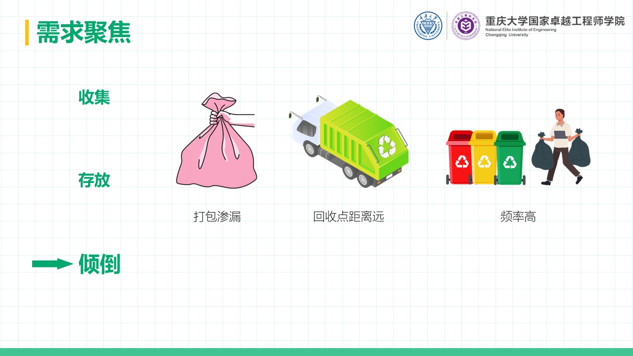
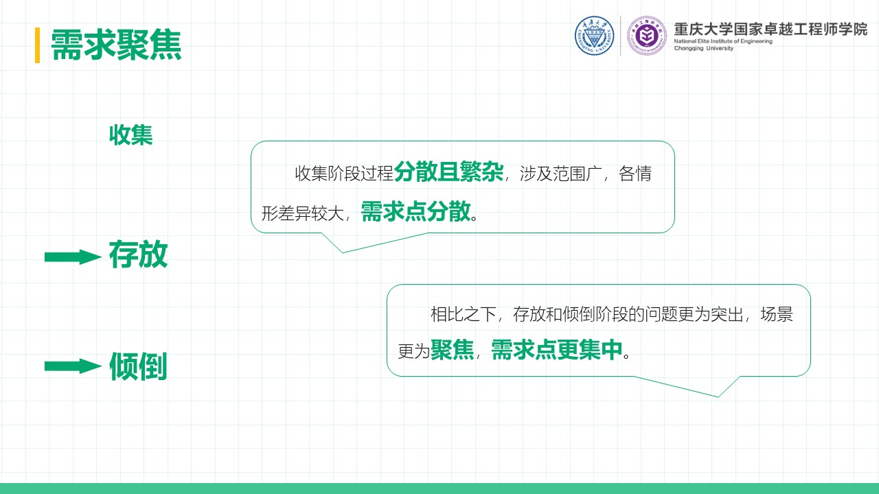
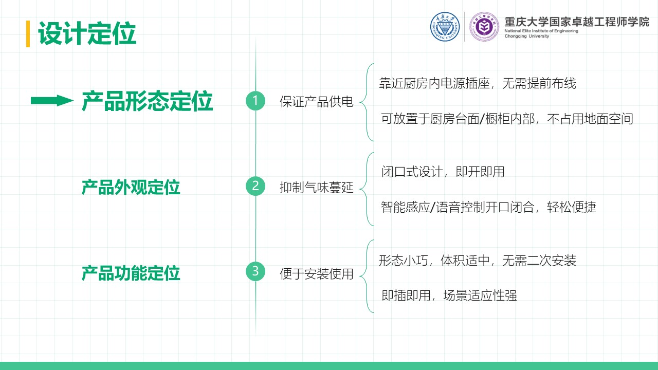
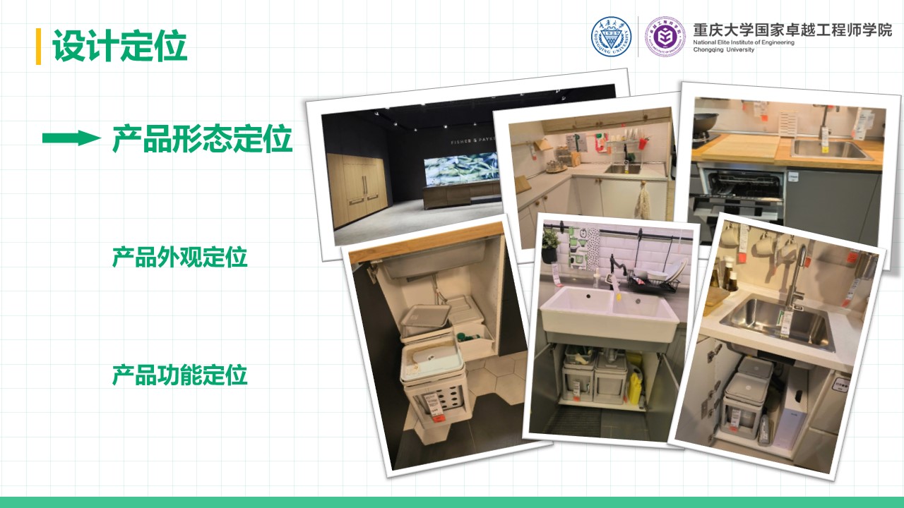
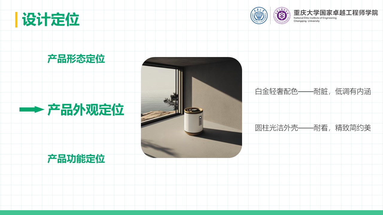
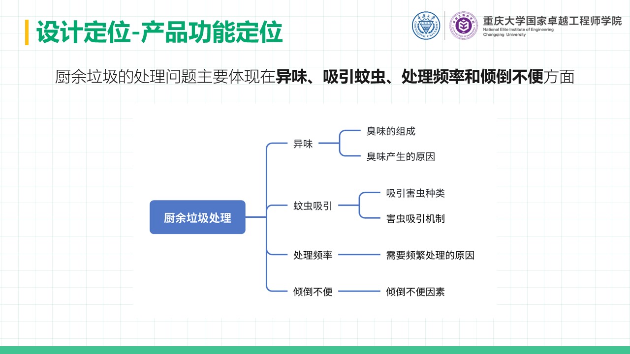
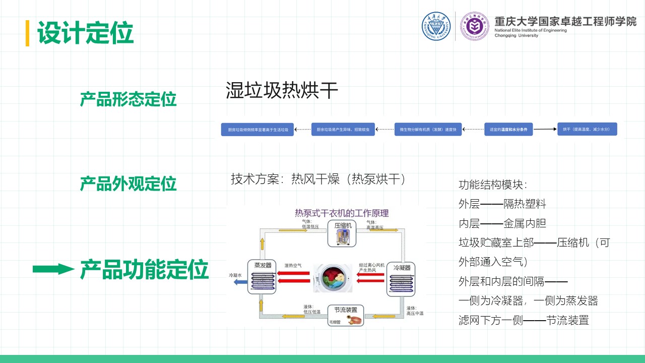
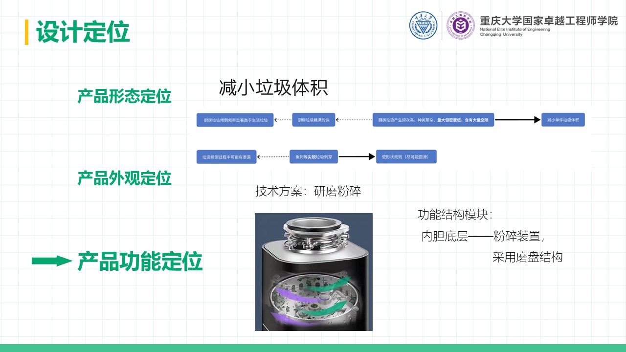
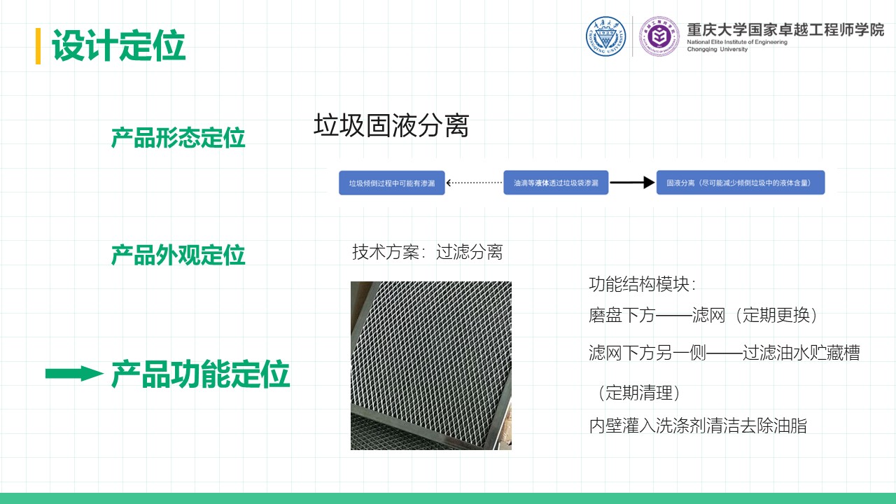
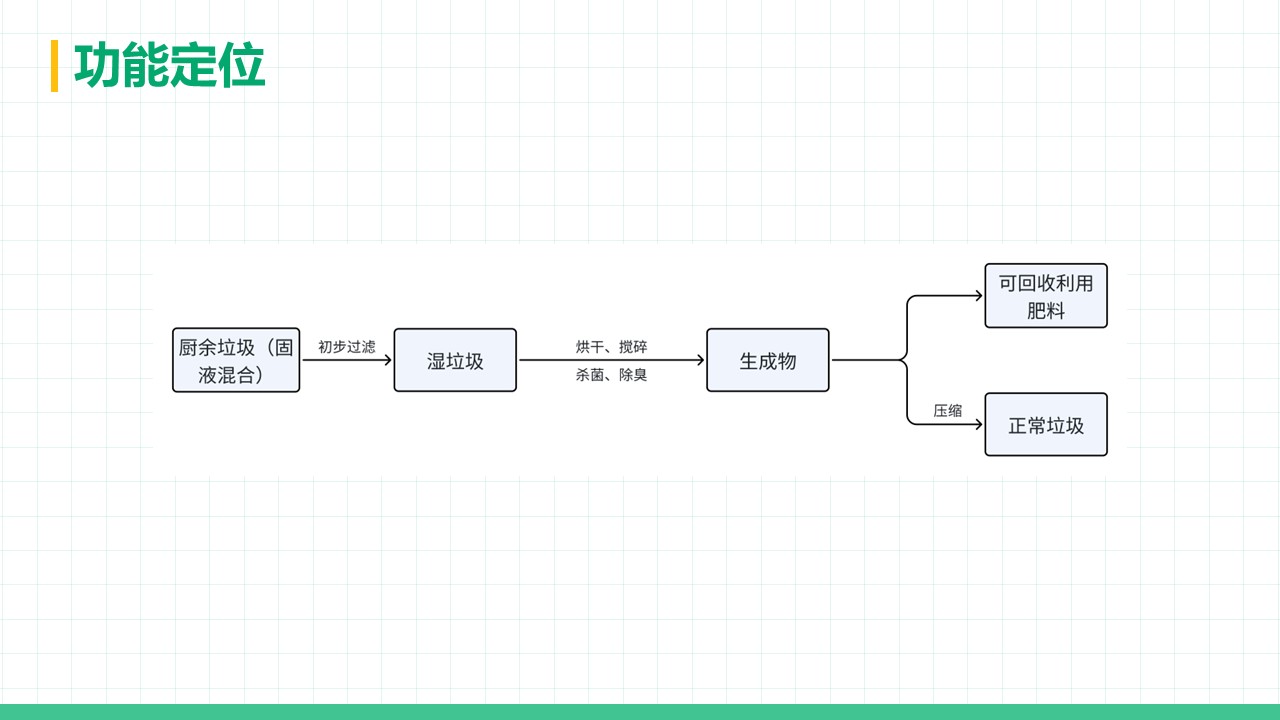
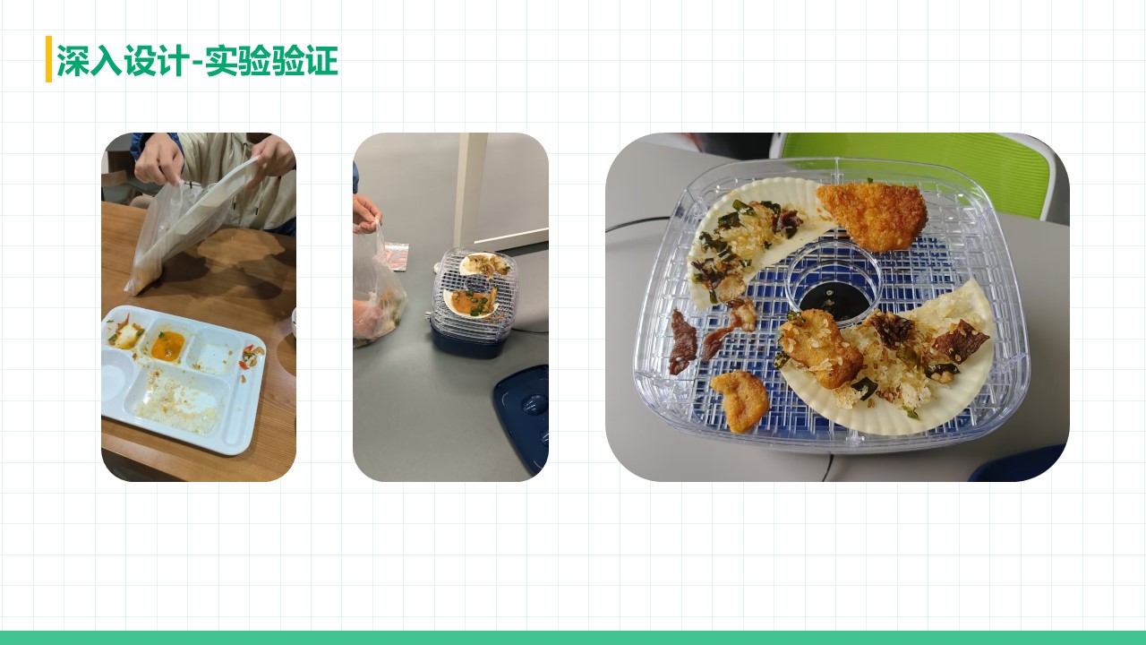
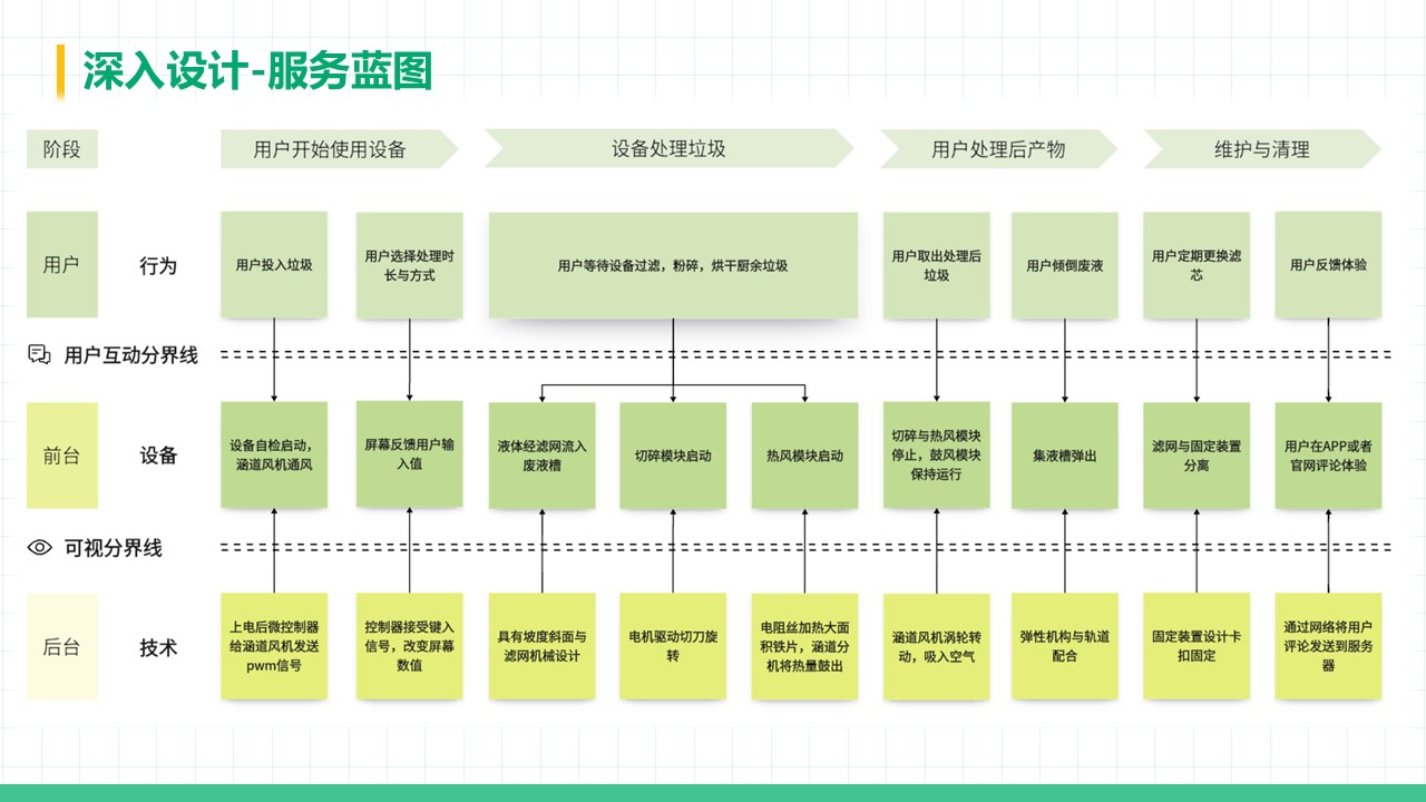
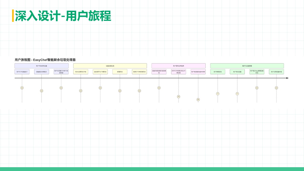
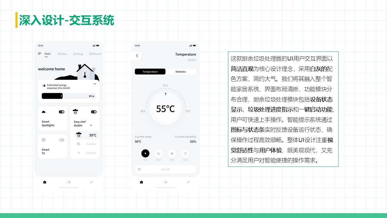
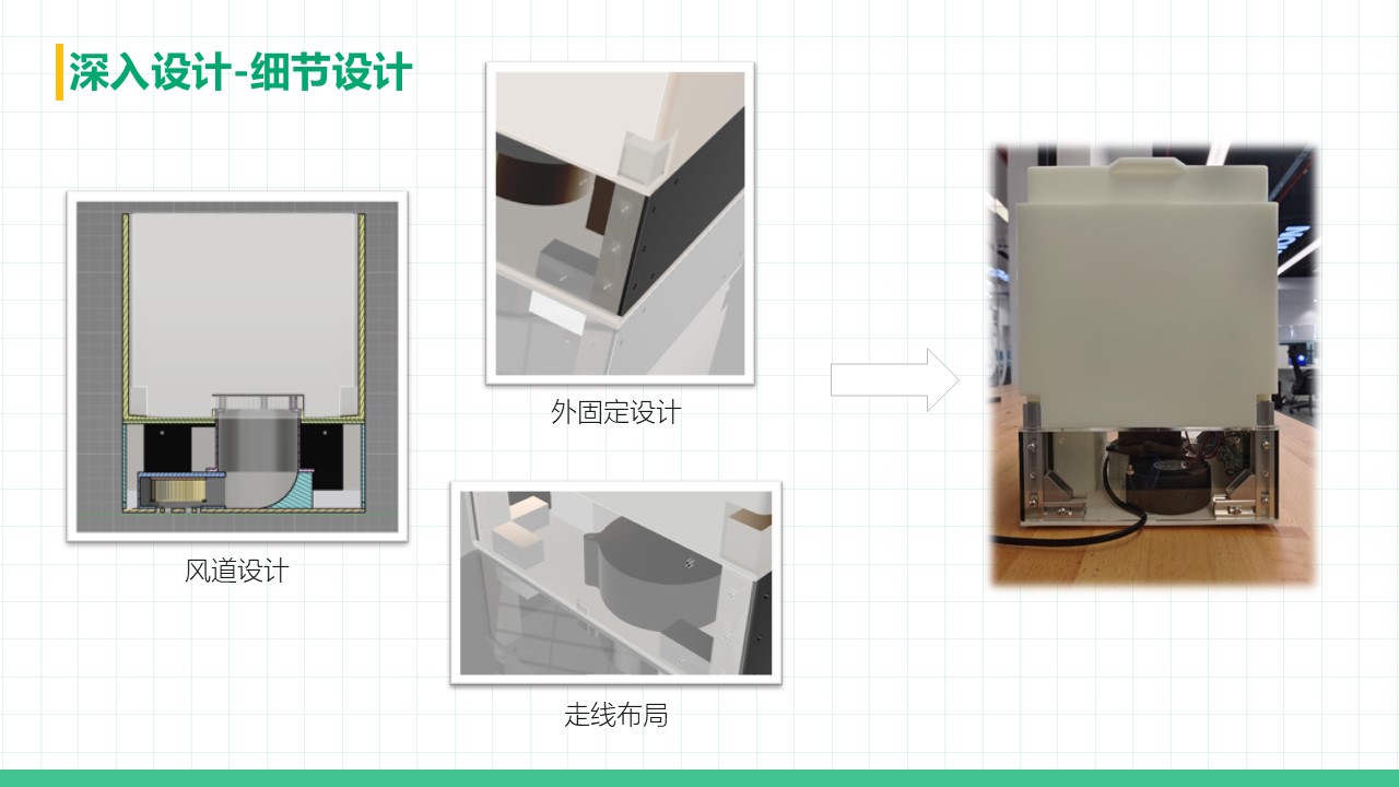
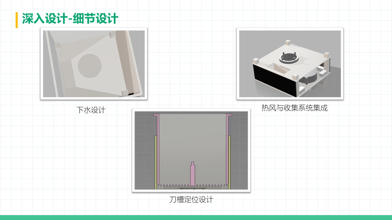
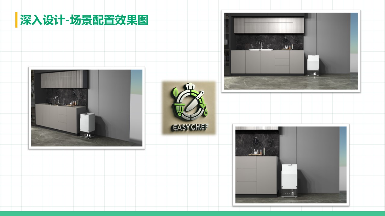
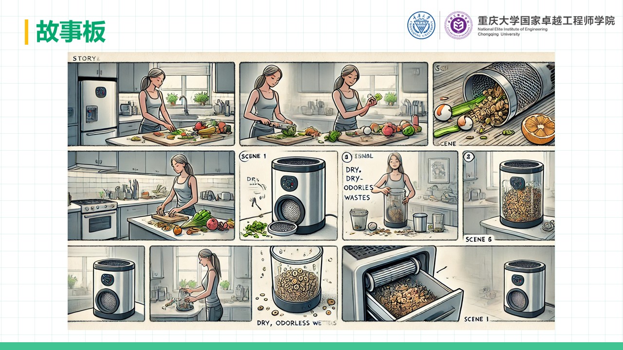
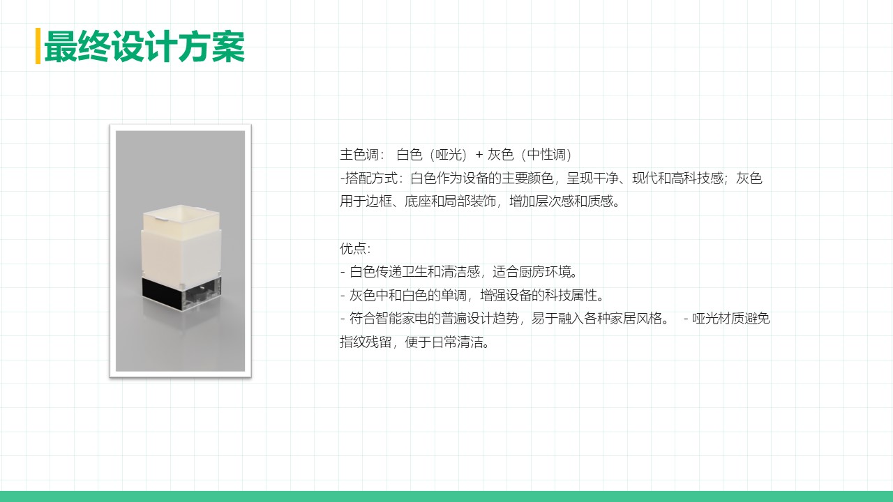
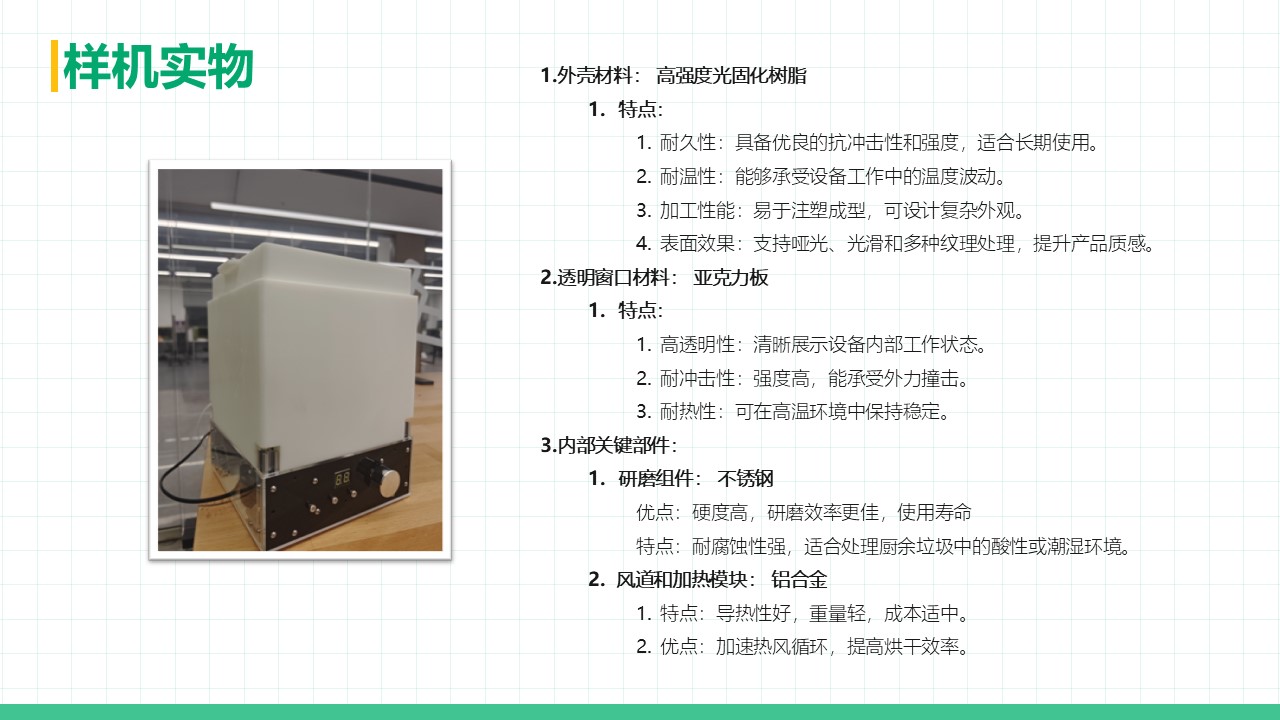
厨余垃圾处理器
以下为课程项目设计产品“厨余垃圾处理器”的结题汇报PPT。
Asgard-Tim
Robotics and Software Engineering
Chongqing Yubei
文章
37
分类
24
标签
102
2025-06-29
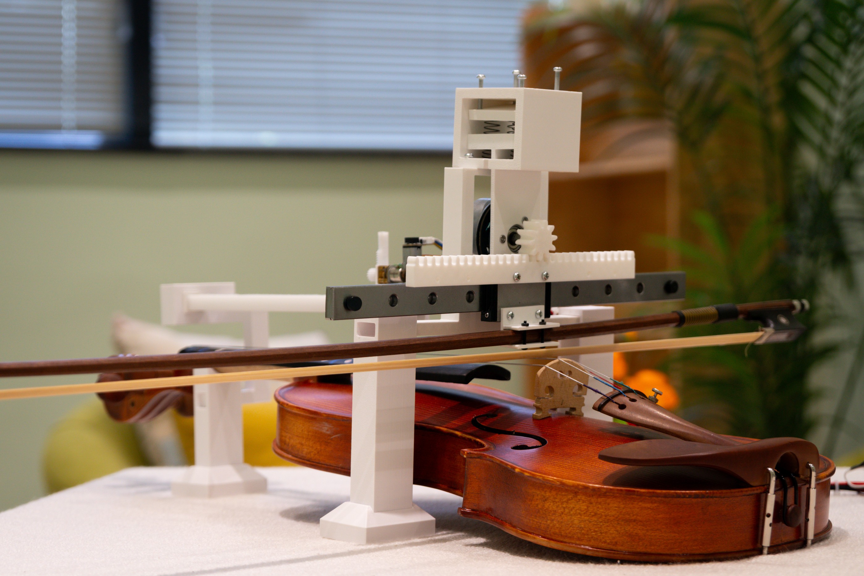
小提琴自动演奏机器人中的齿轮系统设计与制造
课程项目 / 产品制造
2025-06-21
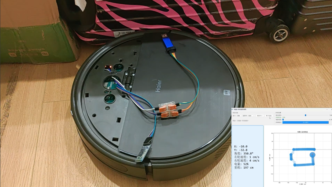
SmartRobot扫地机器人
课程项目 / 微电路设计
2025-06-10
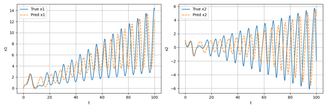
常微分方程反演的机器学习方法
课程项目 / 工程数值分析
2025-05-15
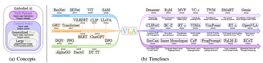
A Survey on Vision-Language-Action Models for Embodied AI
具身智能论文阅读
2025-05-09
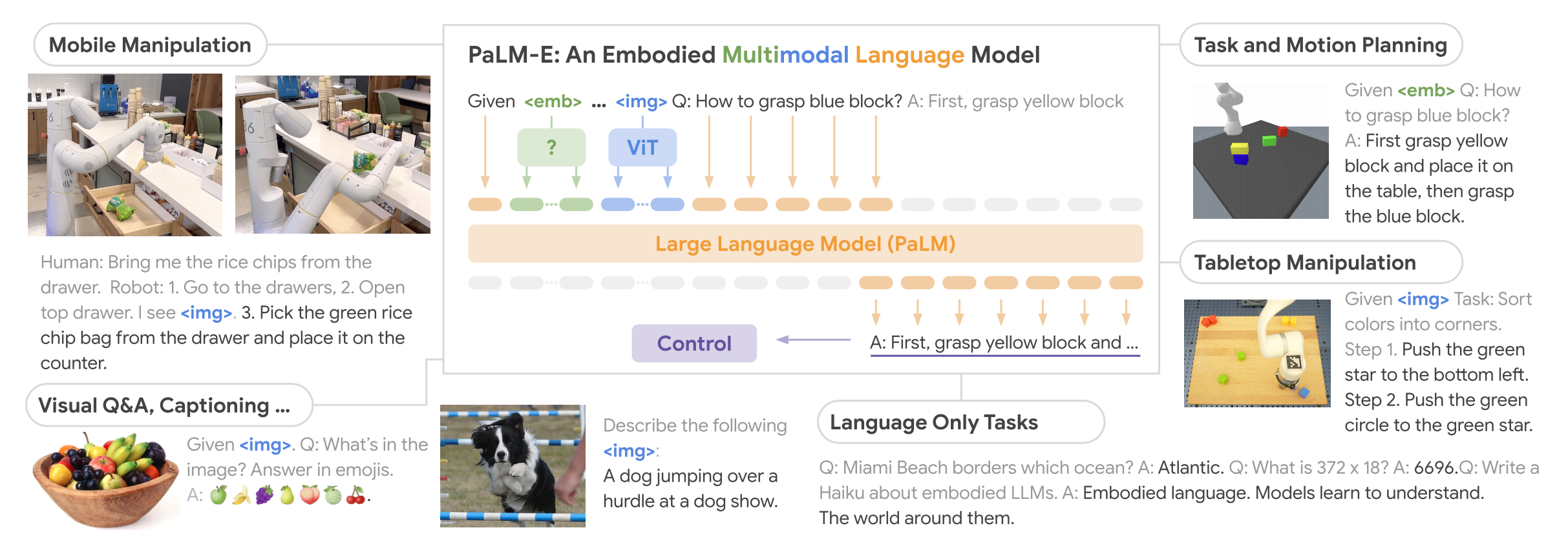
PaLM-E:An Embodied Multimodal Language Model